Flagging Genes (Probesets) Associated with RD in Both TCGA and Tothill
======================================================================
by Keith A. Baggerly
## 1 Executive Summary
### 1.1 Introduction
We want to identify genes whose expression shows
a strong and similarly directed association with
residual disease (RD) status in both the TCGA and Tothill datasets.
### 1.2 Methods
We load our previously assembled RData files for
tcgaExpression,
tcgaFilteredData,
tothillExpression,
tothillFilteredData,
and
tothillClinical.
We restrict our attention to probesets on both
the TCGA and Tothill array platforms.
Then, using just the filtered sets of samples,
we contrast RD and No RD samples within each
dataset using two sample t-tests. For each
probeset in each dataset, we identify the
associated gene and record the mean
expression level in the RD and No RD groups,
the t-statistic, the raw p-value, and the false discovery rate
(FDR) adjusted p-value.
We flag probsets that are significantly different
in both TCGA and Tothill using (a) a 5% FDR cutoff
and (b) a 10% FDR cutoff.
We plot the bivariate t-tests to look for
structure,
expression heatmaps for the selected probes
to look for patterns,
correlations between the probes chosen to
look for coordinated behavior, and
dot and density plots for individual
probesets to identify other features.
We write a convenience function to make
generation of the dot and density plots easier.
### 1.3 Results
There are 22277 probesets common to the two platforms.
We flag 8 probesets using a 5% FDR cutoff in both
datasets,
and 47 probesets using a 10% FDR cutoff.
The bivariate plot of the t-statistics found
is shown in
Figure [1](#bivarTVals); a zoomed version
highlighting the probesets overexpressed in RD samples
is shown in
Figure [2](#bivarTValsZoom).
The expression heatmaps for TCGA and Tothill
using the 5% FDR cutoffs are in
Figures [3](#tcgaHeatmap05pct) and
[4](#tothillHeatmap05pct), respectively.
The expression heatmaps for TCGA and Tothill
using the 10% FDR cutoffs are in
Figures [5](#tcgaHeatmap10pct) and
[6](#tothillHeatmap10pct), respectively.
Heatmaps of the pairwise 10% FDR probe correlations
for TCGA and Tothill are shown in Figures
[7](#tcgaProbesetCors) and [8](#tothillProbesetCors).
Dot and density plots for all 47 probesets passing
the 10% FDR filter are saved as
"plotsOfTop47Probesets.pdf" in the Reports folder.
Dot and density plots for 6 probesets, corresponding to
LUM, DCN, GADD45B, FABP4, ADH1B, and ADIPOQ are
shown in Figures
[9](#lum),
[10](#dcn),
[11](#gadd45b),
[12](#fabp4),
[13](#adh1b), and
[14](#adipoq), respectively.
We save
tcgaCommonUsed,
tothillCommonUsed,
keyProbesets05pct, keyGenes05pct,
keyProbesets10pct, keyGenes10pct,
nTCGANoRD, nTCGARD,
nTothillNoRD, nTothillRD,
plotProbesetResults, and
rdTTestResults
to the RData file "rdFlaggedGenes.RData".
### 1.4 Conclusions
In both sets of expression heatmaps, there is evidence
of a molecularly distinct subset of patients (about a third)
with a higher chance of having RD. Expression levels for most
of the genes identified are consistently higher in these patients.
For LUM, DCN, and GADD45B, which represent the bulk
of the probsets showing elevation, what we see is an
overall mean shift (values are trending higher) without
a clear division point (above here, something's changed).
For FABP4, ADH1B, and (to a lesser extent) ADIPOQ, we
see a *qualitative* shift in a smaller subset -- values for most samples
are very low (effectively "off""), but values for
a subset of patients are very high ("on"").
A qualitative difference strikes us as
more likely to survive a shift across assays
than a mean offset, so we preferentially
pursue FABP4 and ADH1B.
## 2 Libraries
We first load the libraries we will use
in this report.
```r
library(affy)
library(hthgu133a.db)
library(gplots)
```
## 3 Loading the Data
Here we simply load the previously assembled RData files.
clinical information
and expression matrices, and skim the first line of the clinical
information to see what variables exist for filtering the samples.
```r
load(file.path("RDataObjects", "tcgaExpression.RData"))
load(file.path("RDataObjects", "tcgaFilteredSamples.RData"))
load(file.path("RDataObjects", "tothillExpression.RData"))
load(file.path("RDataObjects", "tothillFilteredSamples.RData"))
load(file.path("RDataObjects", "tothillClinical.RData"))
```
## 4 Rearranging Data
### 4.1 Selecting Common Probesets
We only want to examine probesets evaluated in both
datasets.
```r
commonProbesets <- intersect(rownames(tcgaExpression), rownames(tothillExpression))
```
### 4.2 Extracting RD and No RD Samples
Given the common probesets, we next get matrices
of data for RD and No RD measurements for both
TCGA and Tothill.
We begin with TCGA
```r
tcgaCommonRD <- tcgaExpression[commonProbesets, names(tcgaSampleRD)[which((tcgaSampleRD ==
"RD") & (tcgaFilteredSamples[, "sampleUse"] == "Used"))]]
dim(tcgaCommonRD)
```
```
## [1] 22277 378
```
```r
tcgaCommonNoRD <- tcgaExpression[commonProbesets, names(tcgaSampleRD)[which((tcgaSampleRD ==
"No RD") & (tcgaFilteredSamples[, "sampleUse"] == "Used"))]]
dim(tcgaCommonNoRD)
```
```
## [1] 22277 113
```
Next, we repeat the process for Tothill.
```r
tothillCommonRD <- tothillExpression[commonProbesets, names(tothillRD)[which((tothillRD ==
"RD") & (tothillFilteredSamples[, "sampleUse"] == "Used"))]]
dim(tothillCommonRD)
```
```
## [1] 22277 139
```
```r
tothillCommonNoRD <- tothillExpression[commonProbesets, names(tothillRD)[which((tothillRD ==
"No RD") & (tothillFilteredSamples[, "sampleUse"] == "Used"))]]
dim(tothillCommonNoRD)
```
```
## [1] 22277 50
```
### 4.3 Bundling
For later plots, it can be easier to rearrange things
yet again.
```r
tcgaCommonUsed <- cbind(tcgaCommonNoRD, tcgaCommonRD)
tothillCommonUsed <- cbind(tothillCommonNoRD, tothillCommonRD)
```
## 5 Contrasting RD with No RD: T-Tests
### 5.1 Running T-Tests
Our first comparisons involve simple two-sample
t-tests. We perform these for TCGA first.
```r
d1 <- date()
tcgaTVals <- rep(0, length(commonProbesets))
names(tcgaTVals) <- commonProbesets
tcgaPVals <- tcgaTVals
for (i1 in 1:length(commonProbesets)) {
tempT <- t.test(tcgaCommonRD[i1, ], tcgaCommonNoRD[i1, ], var.equal = TRUE)
tcgaTVals[i1] <- tempT[["statistic"]]
tcgaPVals[i1] <- tempT[["p.value"]]
}
d2 <- date()
c(d1, d2)
```
```
## [1] "Wed Nov 20 11:29:41 2013" "Wed Nov 20 11:29:50 2013"
```
```r
tcgaPValsAdj <- p.adjust(tcgaPVals, method = "fdr")
names(tcgaPValsAdj) <- commonProbesets
```
Then we repeat the process with Tothill.
```r
d1 <- date()
tothillTVals <- rep(0, length(commonProbesets))
names(tothillTVals) <- commonProbesets
tothillPVals <- tothillTVals
for (i1 in 1:length(commonProbesets)) {
tempT <- t.test(tothillCommonRD[i1, ], tothillCommonNoRD[i1, ], var.equal = TRUE)
tothillTVals[i1] <- tempT[["statistic"]]
tothillPVals[i1] <- tempT[["p.value"]]
}
d2 <- date()
c(d1, d2)
```
```
## [1] "Wed Nov 20 11:29:50 2013" "Wed Nov 20 11:29:59 2013"
```
```r
tothillPValsAdj <- p.adjust(tothillPVals, method = "fdr")
names(tothillPValsAdj) <- commonProbesets
```
### 5.2 Checking for Overlap at an Extreme Cutoff
We now see which genes (if any) appear significant at
an FDR of 5% in both datasets.
```r
sum(tcgaPValsAdj < 0.05)
```
```
## [1] 149
```
```r
sum(tothillPValsAdj < 0.05)
```
```
## [1] 81
```
```r
sum((tothillPValsAdj < 0.05) & (tcgaPValsAdj < 0.05))
```
```
## [1] 8
```
```r
sum((tothillPValsAdj < 0.1) & (tcgaPValsAdj < 0.1))
```
```
## [1] 47
```
```r
keyProbesets05pct <- names(which((tothillPValsAdj < 0.05) & (tcgaPValsAdj <
0.05)))
keyProbesets10pct <- names(which((tothillPValsAdj < 0.1) & (tcgaPValsAdj < 0.1)))
keyGenes05pct <- unlist(mget(keyProbesets05pct, hthgu133aSYMBOL))
keyGenes10pct <- unlist(mget(keyProbesets10pct, hthgu133aSYMBOL))
keyGenes05pct
```
```
## 201744_s_at 203666_at 203980_at 207574_s_at 209335_at 209613_s_at
## "LUM" "CXCL12" "FABP4" "GADD45B" "DCN" "ADH1B"
## 209687_at 221541_at
## "CXCL12" "CRISPLD2"
```
There are 8 probesets flagged at a common FDR of 5% (listed
above), and 47 probesets flagged at a common FDR of 10%.
### 5.3 Building a Data Frame
Now we bundle our t-test results into a data
frame for later reference, sorting the entries
by mean fdr-adjusted p-value.
```r
tcgaMeanRD <- apply(tcgaCommonRD, 1, mean)
tcgaMeanNoRD <- apply(tcgaCommonNoRD, 1, mean)
tothillMeanRD <- apply(tothillCommonRD, 1, mean)
tothillMeanNoRD <- apply(tothillCommonNoRD, 1, mean)
commonGeneSymbols <- unlist(mget(commonProbesets, hthgu133aSYMBOL))
rdTTestResults <- data.frame(row.names = rownames(tcgaCommonUsed), geneSymbol = commonGeneSymbols,
tcgaMeanRD = tcgaMeanRD, tcgaMeanNoRD = tcgaMeanNoRD, tcgaTVals = tcgaTVals,
tcgaPVals = tcgaPVals, tcgaPValsAdj = tcgaPValsAdj, tothillMeanRD = tothillMeanRD,
tothillMeanNoRD = tothillMeanNoRD, tothillTVals = tothillTVals, tothillPVals = tothillPVals,
tothillPValsAdj = tothillPValsAdj)
rdTTestResults <- rdTTestResults[order(tcgaPValsAdj + tothillPValsAdj), ]
```
As a check, we look at the results for the top 10 probesets
by this ordering.
```r
rdTTestResults[1:10, ]
```
```
## geneSymbol tcgaMeanRD tcgaMeanNoRD tcgaTVals tcgaPVals
## 201744_s_at LUM 9.057 8.084 4.992 8.318e-07
## 203666_at CXCL12 4.400 3.921 4.134 4.202e-05
## 203980_at FABP4 4.278 3.463 3.863 1.272e-04
## 209335_at DCN 7.376 6.746 3.853 1.324e-04
## 209613_s_at ADH1B 3.514 2.944 3.681 2.586e-04
## 221541_at CRISPLD2 6.017 5.444 3.858 1.295e-04
## 209612_s_at ADH1B 3.694 3.196 3.507 4.947e-04
## 207574_s_at GADD45B 6.795 6.392 3.741 2.049e-04
## 209687_at CXCL12 6.885 6.228 3.928 9.811e-05
## 211813_x_at DCN 8.602 8.003 3.525 4.635e-04
## tcgaPValsAdj tothillMeanRD tothillMeanNoRD tothillTVals
## 201744_s_at 0.002885 10.325 9.036 4.536
## 203666_at 0.020107 7.778 6.950 4.160
## 203980_at 0.034264 6.422 4.371 4.533
## 209335_at 0.034609 8.687 7.527 4.560
## 209613_s_at 0.044321 4.912 3.091 5.045
## 221541_at 0.034340 7.523 6.433 4.344
## 209612_s_at 0.057726 5.556 3.781 4.968
## 207574_s_at 0.039855 8.276 7.580 4.155
## 209687_at 0.028758 8.178 7.162 3.986
## 211813_x_at 0.056505 10.921 9.857 4.509
## tothillPVals tothillPValsAdj
## 201744_s_at 1.024e-05 0.010629
## 203666_at 4.842e-05 0.022975
## 203980_at 1.036e-05 0.010629
## 209335_at 9.243e-06 0.010629
## 209613_s_at 1.067e-06 0.002970
## 221541_at 2.289e-05 0.016447
## 209612_s_at 1.521e-06 0.003765
## 207574_s_at 4.937e-05 0.022975
## 209687_at 9.644e-05 0.035837
## 211813_x_at 1.145e-05 0.010629
```
## 6 Plotting Data
Given the contrast results, we now plot the data in several
ways to see if this clarifies aspects of the structure.
### 6.1 Bivariate t-value Plot
Our first check involves plotting the TCGA and Tothill
t-statistics against each other, to see if there are
clear outliers or disagreement with respect to sign.
The initial plot,
Figure [1](#bivarTVals),
shows the vast majority of the probesets selected are
more strongly expressed in RD samples. A zoom on
the upper quadrant of this plot is shown in
Figure [2](#bivarTValsZoom).
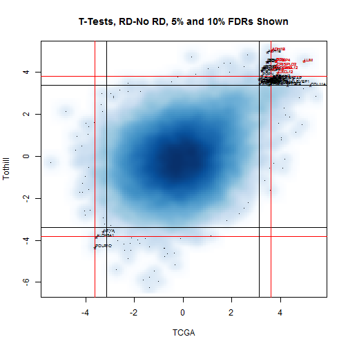
Figure 1: Bivariate plot of two-sample RD-No RD t-values for TCGA and
Tothill. The vast majority of the probesets selected show higher
expression in RD cases. Lumican (LUM) is the strongest overall.
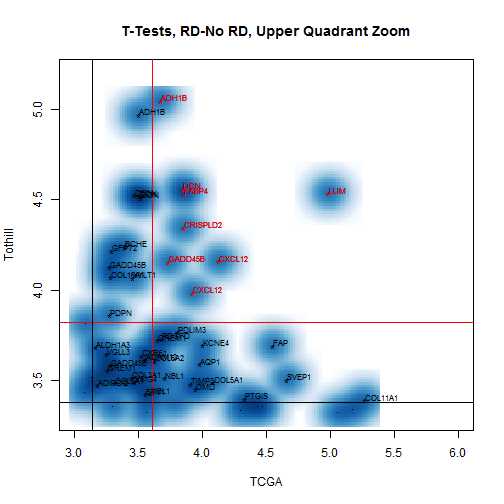
Figure 2: Zoom on the upper quadrant of the
bivariate plot of two-sample RD-No RD t-values for TCGA and
Tothill, to show the names more clearly.
### 6.2 Heatmaps of Probesets Flagged by 5% FDR
We want to see if the most clearly chosen probesets
are flagging the same samples, and how clearly they
divide RD from No RD cases. We check this first
for the 8 probesets passing the 5% FDR filters.
The TCGA heatmap is shown in
Figure [3](#tcgaHeatmap05pct), and
the Tothill heatmap is shown in
Figure [4](#tothillHeatmap05pct).
The general story is the same in both; we see
a clear cluster in which most of the probesets
are concurrently elevated, and the patients in
these clusters have much higher rates of RD.
Of the 8 probesets examined, those for FABP4 and
ADH1B stand out as telling the story most starkly,
though the enrichment rates may not be much higher.
We do not see a tight grouping of the No RD cases,
but this is to be expected since some cases of
RD will not be driven at the molecular level but
rather by spatial positioning in the abdomen.
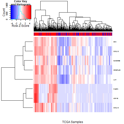
Figure 3: Heatmap of the TCGA Samples using just the 8 probesets passing the
5% FDR filter for both TCGA and Tothill. RD status (Red=RD, Blue=No
RD) is indicated in the colorbar at top. There is a clear cluster
at the left in which most of these genes are concurrently elevated;
the density of RD cases is much higher in this group. Of the probesets
shown, FABP4 and ADH1B stand out from the rest in that they show
a much more marked "on/off" pattern.
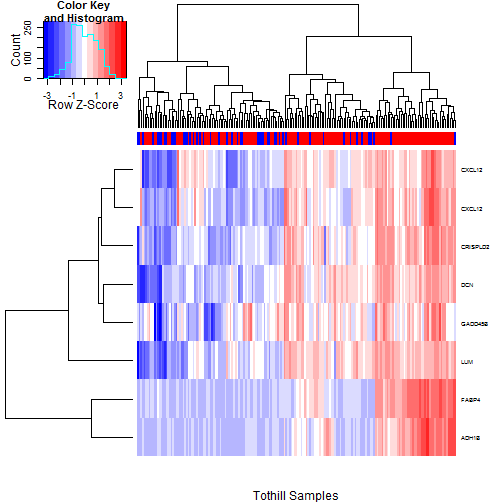
Figure 4: Heatmap of the Tothill Samples using just the 8 probesets passing the
5% FDR filter for both TCGA and Tothill. RD status (Red=RD, Blue=No
RD) is indicated in the colorbar at top. The story essentially
parallels that for the TCGA data.
There is a clear cluster
at the right in which most of these genes are concurrently elevated;
the density of RD cases is much higher in this group. Of the probesets
shown, FABP4 and ADH1B stand out from the rest in that they show
a much more marked "on/off" pattern.
### 6.3 Heatmaps of Probesets Flagged by 10% FDR
Having examined the 5% FDR probesets, we now expand our
view to encompass probesets passing a 10% FDR filter in
both TCGA and Tothill.
The TCGA heatmap is shown in
Figure [5](#tcgaHeatmap10pct), and
the Tothill heatmap is shown in
Figure [6](#tothillHeatmap10pct).
One factor that becomes more apparent here is the
broadly parallel pattern of overexpression seen for
most of the probesets (FABP4 and ADH1B again stand out).
This suggests there may be a common driver for many of
them; possibly a "pathway" of some type.
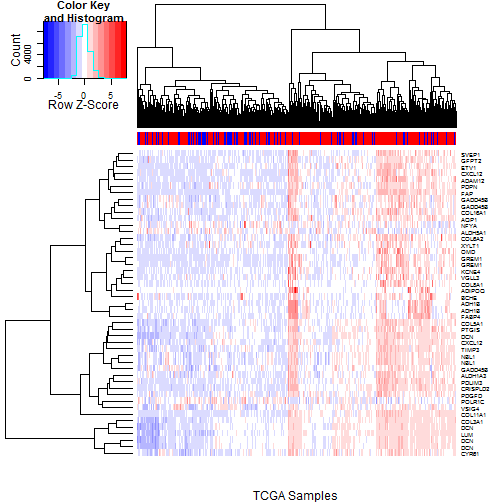
Figure 5: Heatmap of the TCGA Samples using the 47 probesets passing the
10% FDR filter for both TCGA and Tothill. RD status (Red=RD, Blue=No
RD) is indicated in the colorbar at top. While FABP4, ADH1B, and,
to a lesser extent ADIPOQ again stand out, the main visual impression
is one of parallel expression for most of the probesets,
suggesting some common underlying driving factor.
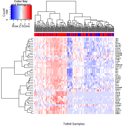
Figure 6: Heatmap of the Tothill Samples using the 47 probesets passing the
10% FDR filter for both TCGA and Tothill. RD status (Red=RD, Blue=No
RD) is indicated in the colorbar at top. As with the TCGA data,
While FABP4, and ADH1B
again stand out, the main visual impression
is one of parallel expression for most of the probesets,
suggesting some common underlying driving factor.
### 6.4 Heatmaps of Correlation of Probesets Flagged by 10% FDR
Given the broad parallelism of expression seen in the heatmaps of
probesets passing the 10% FDR filters, we want to check the
correlation patterns between these probes.
The TCGA heatmap is shown in
Figure [7](#tcgaProbesetCors), and
the Tothill heatmap is shown in
Figure [8](#tothillProbesetCors).
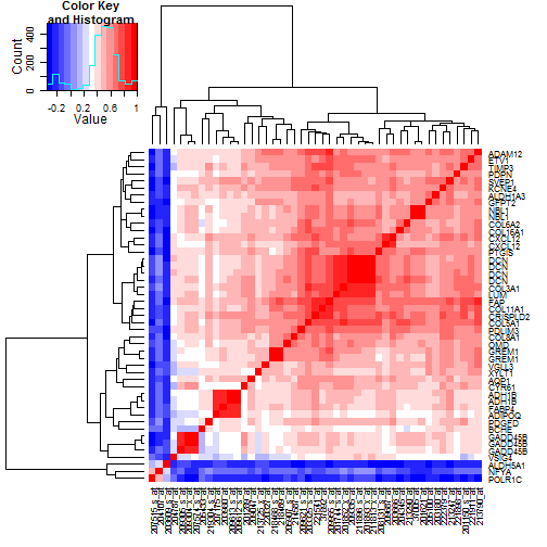
Figure 7: Correlations in the TCGA data between the
47 probesets selected by 10% FDR cutoffs. While
the three probesets where expression declines
drive the coloring most, the main story in terms
of commonality may be the grouping of 26
probesets in the upper right, including lumican (LUM)
and decorin (DCN). Cutting the probsets into three
clusters overall,
FABP4 and ADH1B reside in the second
grouping of probesets at the right.
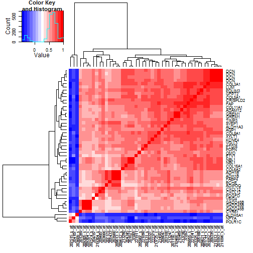
Figure 8: Correlations in the Tothill data between the
47 probesets selected by 10% FDR cutoffs. While
the three probesets where expression declines
drive the coloring most, the main story in terms
of commonality may be the tight grouping of 31
probesets in the upper right, including lumican (LUM)
and decorin (DCN). FABP4 and ADH1B reside in the second
grouping of probesets at the right.
### 6.5 Density Plots and Dotplots
We know some of the probesets are of interest.
Now we look at aspects of behavior of the individual
probesets, specifically dotplots and density plots
for each probeset by dataset.
First, we construct a generic function for plotting
these results for a given probeset.
```r
plotProbesetResults <- function(probesetID) {
par(mfrow = c(2, 2))
geneName <- unlist(mget(probesetID, hthgu133aSYMBOL))
plot(tcgaCommonUsed[probesetID, ], col = c(rep("blue", nTCGANoRD), rep("red",
nTCGARD)), xlab = "TCGA Samples", ylab = "Expression", main = paste("Expression of",
geneName, "in TCGA"))
abline(v = nTCGANoRD + 0.5)
plot(tothillCommonUsed[probesetID, ], col = c(rep("blue", nTothillNoRD),
rep("red", nTothillRD)), xlab = "Tothill Samples", ylab = "Expression",
main = paste("Expression of", geneName, "in Tothill"))
abline(v = nTothillNoRD + 0.5)
tempDensTCGA <- density(tcgaCommonUsed[probesetID, ])
tempDensTCGANoRD <- density(tcgaCommonNoRD[probesetID, ])
tempDensTCGARD <- density(tcgaCommonRD[probesetID, ])
plot(tempDensTCGA[["x"]], tempDensTCGA[["y"]], xlab = paste("Expression of",
probesetID, "in TCGA"), ylab = "Density", type = "l", main = paste("Density of",
probesetID, "in TCGA"))
lines(tempDensTCGANoRD[["x"]], (nTCGANoRD/(nTCGANoRD + nTCGARD)) * tempDensTCGANoRD[["y"]],
col = "blue")
lines(tempDensTCGARD[["x"]], (nTCGARD/(nTCGANoRD + nTCGARD)) * tempDensTCGARD[["y"]],
col = "red")
tempDensTothill <- density(tothillCommonUsed[probesetID, ])
tempDensTothillNoRD <- density(tothillCommonNoRD[probesetID, ])
tempDensTothillRD <- density(tothillCommonRD[probesetID, ])
plot(tempDensTothill[["x"]], tempDensTothill[["y"]], xlab = paste("Expression of",
probesetID, "in Tothill"), ylab = "Density", type = "l", main = paste("Density of",
probesetID, "in Tothill"))
lines(tempDensTothillNoRD[["x"]], (nTothillNoRD/(nTothillNoRD + nTothillRD)) *
tempDensTothillNoRD[["y"]], col = "blue")
lines(tempDensTothillRD[["x"]], (nTothillRD/(nTothillNoRD + nTothillRD)) *
tempDensTothillRD[["y"]], col = "red")
par(mfrow = c(1, 1))
}
```
For reference, we produce a pdf file containing the results
for all 47 probesets in our top list.
```r
pdf(file = file.path("Reports", "plotsOfTop47Probesets.pdf"))
for (i1 in 1:length(keyProbesets10pct)) {
plotProbesetResults(keyProbesets10pct[i1])
}
dev.off()
```
```
## pdf
## 2
```
We include results for a few selected genes here:
LUM (201744\_s\_at), Figure [9](#lum),
DCN (211896\_s\_at), Figure [10](#dcn),
GADD45B (207574\_s\_at), Figure [11](#gadd45b),
FABP4 (203980\_at), Figure [12](#fabp4),
ADH1B (209613\_s\_at), Figure [13](#adh1b), and
ADIPOQ (207175\_at), Figure [14](#adipoq).
For some of the genes (ADH1B, DCN), mutliple probesets
are available but the results appear qualitatively similar
to the representative ones chosen.
For LUM, DCN, and GADD45B, which represent the bulk
of the probsets showing elevation, what we see is an
overall mean shift (values are trending higher) without
a clear division point (above here, something's changed).
For FABP4, ADH1B, and (to a lesser extent) ADIPOQ, we
see a qualitative shift -- values for most samples
are very low (effectively "off""), but values for
a subset of patients are very high ("on"").
This type of qualitative difference strikes us as
more likely to survive a shift across assays
than a mean offset, so we will preferentially
pursue FABP4 and ADH1B.
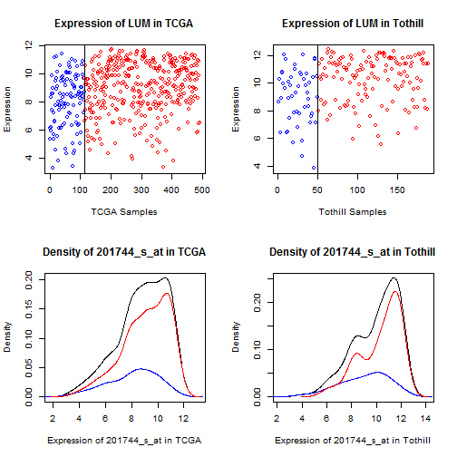
Figure 9: Dot and density plots for lumican (LUM) in TCGA
and Tothill. Cases with No RD are blue, RD are red.
While there is a clear mean shift (which drives the
t-test results), there is not a clearly defined
cutpoint.
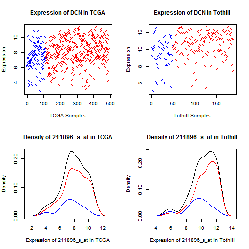
Figure 10: Dot and density plots for decorin (DCN) in TCGA
and Tothill. Cases with No RD are blue, RD are red.
While there is a clear mean shift (which drives the
t-test results), there is not a clearly defined
cutpoint.
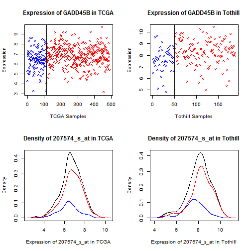
Figure 11: Dot and density plots for GADD45B in TCGA
and Tothill. Cases with No RD are blue, RD are red.
While there is a clear mean shift (which drives the
t-test results), there is not a clearly defined
cutpoint.
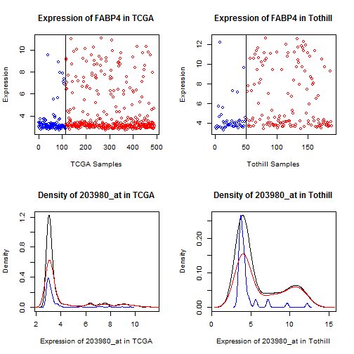
Figure 12: Dot and density plots for FABP4 in TCGA
and Tothill. Cases with No RD are blue, RD are red.
There is a qualitative shift in a subset of the patients.
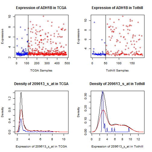
Figure 13: Dot and density plots for ADH1B in TCGA
and Tothill. Cases with No RD are blue, RD are red.
There is a qualitative shift in a subset of the patients.
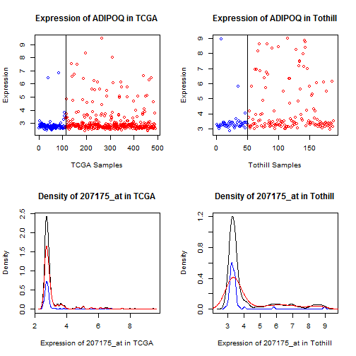
Figure 14: Dot and density plots for ADIPOQ in TCGA
and Tothill. Cases with No RD are blue, RD are red.
There is a qualitative shift in a subset of the patients.
## 7 Saving RData
Now we save the relevant information to an RData object.
```r
save(tcgaCommonUsed, tothillCommonUsed, keyProbesets05pct, keyGenes05pct, keyProbesets10pct,
keyGenes10pct, nTCGANoRD, nTCGARD, nTothillNoRD, nTothillRD, plotProbesetResults,
rdTTestResults, file = file.path("RDataObjects", "rdFlaggedGenes.RData"))
```
## 8 Appendix
### 8.1 File Location
```r
getwd()
```
```
## [1] "/Users/slt/SLT WORKSPACE/EXEMPT/OVARIAN/Ovarian residual disease study 2012/RD manuscript/Web page for paper/Webpage"
```
## 8.2 SessionInfo
```r
sessionInfo()
```
```
## R version 3.0.2 (2013-09-25)
## Platform: x86_64-apple-darwin10.8.0 (64-bit)
##
## locale:
## [1] en_US.UTF-8/en_US.UTF-8/en_US.UTF-8/C/en_US.UTF-8/en_US.UTF-8
##
## attached base packages:
## [1] parallel stats graphics grDevices utils datasets methods
## [8] base
##
## other attached packages:
## [1] gplots_2.12.1 hthgu133a.db_2.9.0 org.Hs.eg.db_2.9.0
## [4] RSQLite_0.11.4 DBI_0.2-7 AnnotationDbi_1.22.6
## [7] affy_1.38.1 Biobase_2.20.1 BiocGenerics_0.6.0
## [10] knitr_1.5
##
## loaded via a namespace (and not attached):
## [1] affyio_1.28.0 BiocInstaller_1.10.4 bitops_1.0-6
## [4] caTools_1.14 evaluate_0.5.1 formatR_0.9
## [7] gdata_2.13.2 gtools_3.1.0 IRanges_1.18.4
## [10] KernSmooth_2.23-10 preprocessCore_1.22.0 stats4_3.0.2
## [13] stringr_0.6.2 tools_3.0.2 zlibbioc_1.6.0
```