TCGA Batch Effects Viewer

| Overview | |
| Description | The TCGA Batch Effects website analyzes TCGA data and provides quantitative and visual means for users to identify and quantify the amount of batch effect present in a given TCGA data set. |
| Development Information | |
| URL | http://bioinformatics.mdanderson.org/tcgambatch/ |
| Language | D3 (JS), Dojo 1.7(JS), Java |
| Current version | 2.0 |
| Status | Active |
| Last updated | Released |
| News | Data for 21 different tumor types are now available |
| Help and Support | |
| Contact | Rehan Akbani |
| Discussion | On GitHub |
TCGA Batch Effects Viewer
A large, complex, multi-faceted, multi-institutional project such as The Cancer Genome Atlas (TCGA) collects tumor samples in different institutions and at different times. Because the samples are processed in batches rather than all at once, the data can be vulnerable to systematic noise such as batch effects (unwanted variation between batches) and trend effects (unwanted variation over time), which can lead to misleading analysis results.
This website is designed to help assess, diagnose and correct for any batch effects in TCGA data. It first allows the user to assess and quantify the presence of any batch effects via algorithms such as Hierarchical Clustering and Principal Component Analysis. The results from these algorithms are presented graphically as both simple and interactive diagrams. If significant batch effects is observed in the data, the user then has the option of downloading data that has been computationally corrected using methods such as Empirical Bayes (aka. ComBat), Median Polish and ANOVA.
The website is currently under development, so only a subset of TCGA level 3 data has been analyzed thus far. Our eventual goal is to completely and comprehensively annotate all TCGA data sets, and provide users with batch effects corrected data for all of them.
Before using TCGA data, please read TCGA guidelines for publication and moratoriums .
LAUNCH TCGA BATCH EFFECTS WEBSITE
See also the MBatch R package.
TCGA Data Collection Process
Below is a quick overview of the various steps involved in the TCGA Data Collection Process, each of which could potentially introduce systematic errors. Relevant terms are highlighted in bold and explanatory links have been provided wherever possible.
- Biospecimens consisting of Tumor and Normal tissue samples and clinical metadata are collected from patients donors at various Tissue Source Sites (TSS). Each TSS is identified by its unique TSS ID.
- These biospecimens are transported to TCGA Biospecimen Core Resources (BCR) laboratories, which ensure these specimens meet the TCGA biospecimen criteria . Specimens of sufficient quality are cataloged, processed and stored for analysis. Any patient identifying information is removed during the process.
- Specimens are grouped into batches consisting of a fixed set of patient cases of the same disease study. Each batch is uniquely determined by the first shipment of a group of analytes from the Biospecimen Core Resource.
- Analytes are transported to sequencing centers on various ShipDates and processed into usable data on plates each with its own unique PlateID.
- This data are then sent to TCGA Genome Characterization Centers and Genome Sequencing Centers (CGCC and GSC) for interpretation.
- TCGA Genome Characterization Centers analyze many of the genetic changes involved in cancer including how the genome is rearranged or how gene expression changes in tumors compared to normal cells.
- High-throughput TCGA Genome Sequencing Centers identify the changes in DNA sequence associated with specific types of cancer.
- The information that is generated by the TCGA Research Network is centrally managed at the TCGA Data Coordinating Center and made available on the TCGA Data Portal by release date.
Quantitative measures of Batch Effects
The DSC metric
Dispersion Separability Criterion (DSC) is a new metric that has been designed to quantify the amount of batch effect in the data. It is based on a similar metric, the Scatter Separability Criterion. DSC is defined as:
$$DSC = D_b/D_w$$
Where $D_b$ is a measure of dispersion between batches (or other groupings of the data), and $D_w$ is a measure of dispersion within batches. Therefore, DSC is a ratio of between batch dispersion vs. within batch dispersion. More precisely, $D_b$ is defined as:
$$ D_b = \sqrt{trace(S_b)} $$
and $D_w$ is defined as:
$$ D_w = \sqrt{trace(S_w)} $$
Where $S_b$ is the “between batch” scatter matrix, and Sw is the “within batch” scatter matrix defined in Dy et al, 2004 . $D_w$ can roughly be viewed as the average “distance” between samples within a batch and the batch mean, or centroid, whereas $D_b$ can roughly be viewed as the average distance between batch centroids and the global mean.
Interpretation
A higher DSC value means that there is a greater dispersion between batches than within batches, i.e. the samples within batches are more homogeneous to each other than the batches themselves are to each other. It is a continuous positive number and as such, there is no absolute threshold where one could binarize the results, so that values above the threshold indicate a batch effect and vice versa. However, as a rule of thumb, for DSC values significantly below 0.5, one can usually assume that batch effects aren’t very strong. Values above 0.5 indicate that one needs to consider the possibility of batch effects existing in the data. Values above 1 usually indicate strong batch effects that may need to be corrected before the data can be used for analysis. However, one also needs to consider the DSC p-value before making such an assessment.
DSC p-value
Batches can sometimes contain outliers that may skew the DSC value, since the value is based on taking averages. This may especially be a problem when the batch sizes are small. To counter that possibility, another metric, the DSC p-value, is provided to aid researchers in assessing the statistical significance of the DSC value. The p-value is derived empirically, using permutation tests. One thousand or more permutations are typically run on each data set, using different random permutations of the data each time. DSC values are computed for each permutation and at the end of all the runs, the proportion of values greater than the actual DSC value is computed to yield the p-value. The null hypothesis is that there are no batch effects and the data set is homogeneous in terms of batches. A p-value less than some significance threshold (usually 0.05) rejects the null hypothesis.
However, it should be noted that large enough sample sizes can yield significant p-values even though the overall difference between batches may be very small. This is typical of most p-value based hypothesis testing. Therefore, we recommend that both p-value as well as the DSC value itself be used to assess whether batch effects are are present in the data or not. Batch effects would be expected to be present if the p-value were significant (less than 0.05 for example) AND the DSC value was high (greater than 0.5 for instance). If either of those conditions was false, batch effects can be presumed to be less serious.
Correction of Batch Effects
The website provides data that has been corrected for batch effects. Users will have the choice to assess the amount of batch effects in the original TCGA data, and if they feel that the batch effects are significant, they can download computationally corrected data. The corrected data is computed using the Empirical Bayes (aka.Combat), Median Polish and ANOVA. Batch effects assessment results after correction will be made available for each method to allow users to make an informed decision about which data sets they want to use for their analyses.
Basic Layout
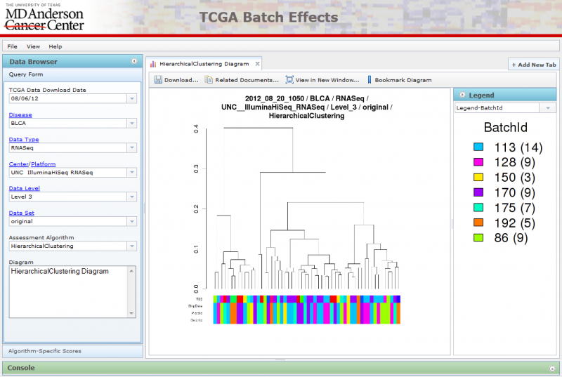
The Menu allows you to control viewing options and gain access to website documentation.
The Data Browser on the left provides various means to select data for viewing. The query form allows one to select data by standard TCGA data fields such as Disease Type, Center/Platform, Data Level and Data Set. The Algorithmic-specific scores allows one to zoom in on data sets that registered particularly high DSC scores. The Data Browser can be hidden to allow for more space to view the diagrams.
The Tabbed Viewing Area in the bottom right allows one to open multiple diagrams and tables at once.
The Console at the bottom currently does not do anything, but will show additional textual information in the future.
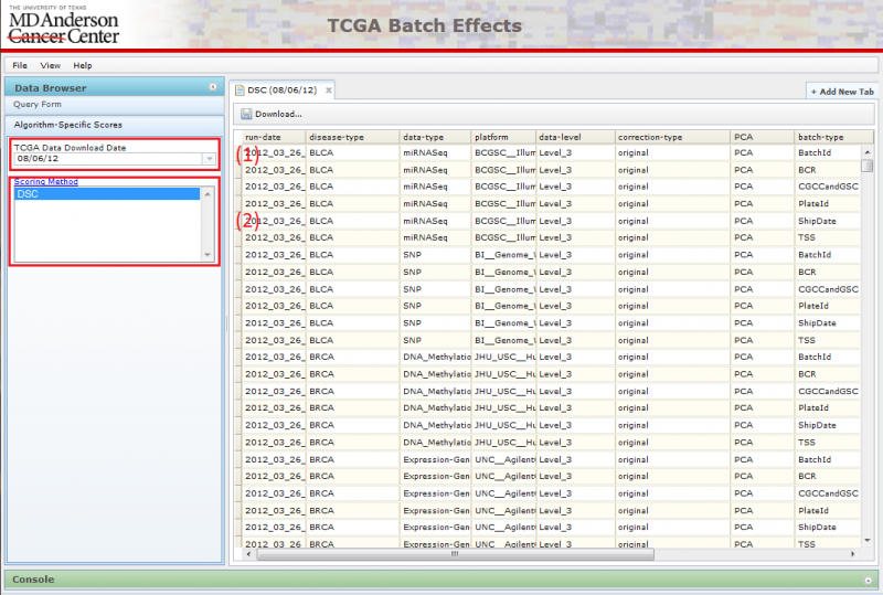
Navigating Data Sets using the Query Form
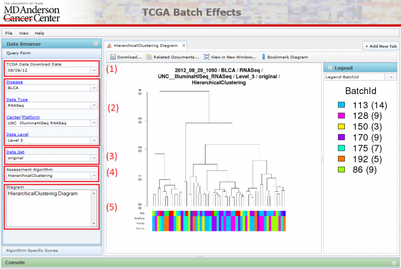
Parts (1), (2), (3), (4), (5) together forms the Query Form on the left. The Query Form consists of a number of select boxes that allows the user to navigate through the different diagrams by choosing properties related to the data set and assessment algorithm. The page refreshes when the user makes a change to any one of the select boxes, and the diagram image and the accordion menu on the right will be updated correspondingly.
(1) Pick the TCGA download date.
- When you first arrive on the website, the latest TCGA data is chosen by default.
(2) Locate the dataset you are interested in examining by setting the following parameters:
- Disease: Choose the cancer tissue type.
- Data Type: Choose the type of data you are interested in.
- Center/Platform: Choose the Center and the Technology used for measuring the data.
- Data Level: Choose the data level
(3) Choose between viewing original data and corrected data
- Original Data: Data filtered to remove data points with missing values
- Corrected Data: Data corrected to account for batch effects via various methods
(4) Select an assessment algorithm
(5) Pick settings that are custom to the assessment algorithm type.
Navigating Data Sets using Algorithm-Specific Scores
You can identify data showing large batch effects quantitatively by using the Algorithm-Specific Scores pane in the Data Browser. Currently, only DSC scores are available for viewing.
To use this interface:
(1) Pick the TCGA download date.
- When you first arrive on the website, the latest TCGA data is chosen by default.
(2) Pick the Algorithm-Specific Score.
- Currently only DSC is available.
Picking the score type will launch the corresponding table on the right. You can sort the data by clicking on the header of the column you wish to sort by. Repeated clicks on the same column header will alternate the sort between ascending and descending order.
Viewing Hierarchical Clustering Diagrams
Hierarchical Clustering diagrams groups samples together based on similarity.
There are often multiple legends associated with each Hierarchical Clustering image, one associated with each row at the bottom of the diagram. You can select the legend you want using the combobox underneath the legend panel on the right. You can also hide the legend panel by clicking on the small circular arrow button within the Blue ‘Legend’ title.
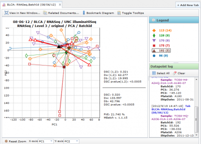
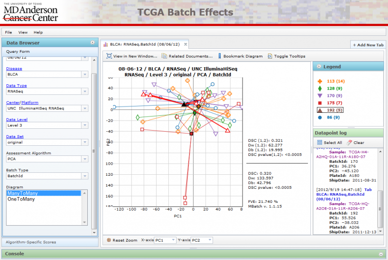
Viewing Principal Component Analysis Diagrams
u can view scatter plots of the first 4 components of PCA analysis on the interactive PCA diagrams.
There are two types of PCA diagrams you can pick using the query form:
ManyToMany PCA Diagrams
All available batches are plotted against one another.
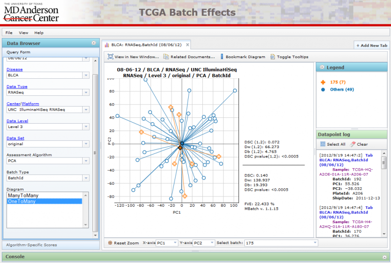
OneToMany PCA Diagrams
A single batch can be selected using the ‘Select batch’ combobox at the bottom, while all other batches are grouped together using a single color.
Interactive Features
You can zoom in/out of the diagram by using the mouse scroll wheel. Double-clicking on the diagram will cause the diagram to zoom in as well.
You can pan the diagram by clicking and dragging across the canvas.
You can pick the PCA components you want to plot using the x-axis and y-axis comboboxes below.
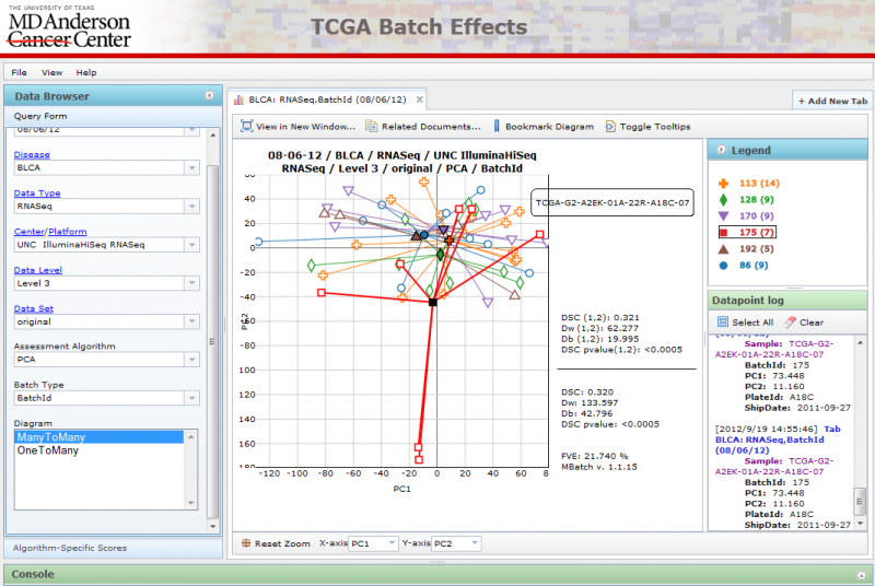
To view details for each point, mouse over the points and wait for a second. The details of the points will appear in the Datapoint log in the lower right, and the group that the datapoint belows to will be highlighted in the Legend. Mousing over the centroid will highlight the entire group.
You can also optionally display a popup label for the point by using the ‘Toggle Tooltips’ button at the top.
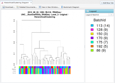
Opening Diagrams in New Windows
You can open a diagram in a new window if you wish to compare 2 diagrams side by side by clicking on the ‘View in New Window’ button. This will launch the diagram in a new window:
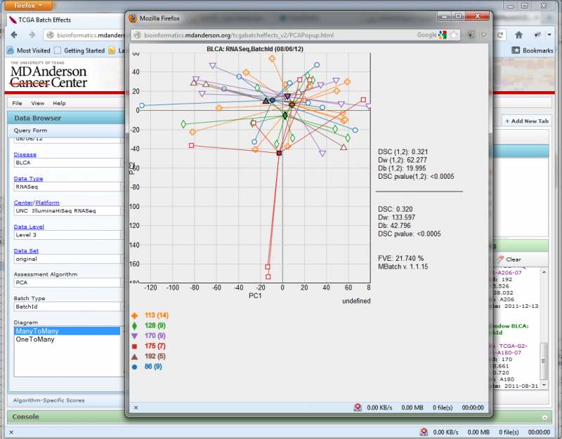
Resizing the window will automatically change the diagram size to match.
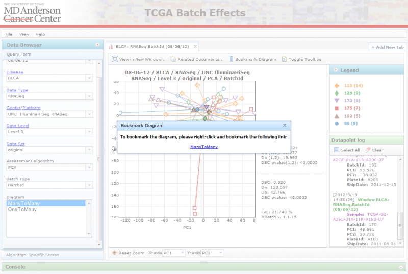
Bookmarking Diagrams
You can bookmark a diagram to revisit later, or to share with other users, by clicking on the ‘Bookmark’ button. This will launch a dialog box with a link on it. To bookmark the diagram, right-click on the link and add it to your bookmarks (may vary across browsers). To share the diagram with other users, right-click on the link, copy the url and share it with others.
Viewing Related Files
When you click on “Related Documents”, you can see a list of files associated with the chosen diagram and data set:
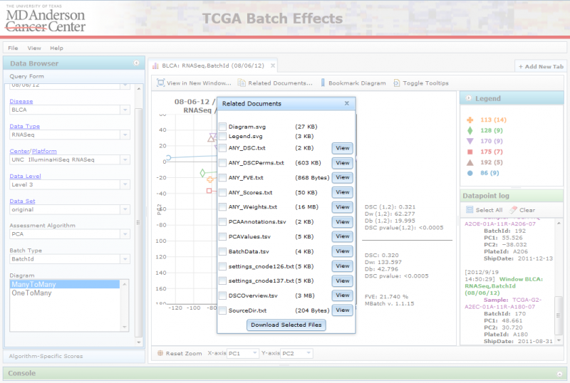
To download the files, mark the checkboxes for the ones you are interested in, and click on the ‘Download Selected Files’ button. This will download a zip file to your computer containing the selected files. Alternatively, you can also view certain files on the website itself using the file’s ‘View’ button. This will launch a separate tab displaying its contents.
File Types
A detailed description of each file type is given below:
Files available with all diagrams
The following files are available for download on all plot typen.
*_Diagram.zip
- A zip file containing the displayed diagram image packaged together with all relevant legends.
Files specific to PCA diagrams
The following text files are available for viewing or download with all PCA plots.
ANY_Comp1_Comp2_DSC.txt: This file contains the following information:
- The number of the first principal component shown in the associated figure.
- The Fraction of Variation Explained (FVE) by that component (as a percentage).
- The number of the second principal component shown in the figure.
- The Fraction of Variation Explained (FVE) by that component (as a percentage).
- The Dispersion Separability Criterion (DSC) metric for the pair of components shown in the figure (see DSC description above).
- The between group dispersion metric (DB) for the pair of components shown in the figure (see DB description above).
- The within group dispersion metric (DW) for the pair of components shown in the figure (see DW description above).
- The p-value associated with the DSC metric for the pair of components shown in the figure (see DSC description above).
- The Dispersion Separability Criterion (DSC) metric over the entire data set (i.e. all the principal components).
- The between group dispersion metric (DB) over the entire data set.
- The within group dispersion metric (DW) over the entire data set.
- The p-value associated with the DSC metric over the entire data set.
ANY_DSC.txt: This tab separated file has 6 columns:
- Column 1: Principal component number
- Column 2: (FVE) Fraction of Variation Explained (FVE) by that component (as a percentage)
- Column 3: (DSC) The value of the Dispersion Separability Criterion (DSC) metric for that component (see DSC description above)
- Column 4: (DB) The value of the between group dispersion metric for that component (see DB description above)
- Column 5: (DW) The value of the within group dispersion metric for that component (see DW description above)
- Column 6: The p-value associated with the DSC metric for that component (see DSC description above)
ANY_FVE.txt: This tab separated file has 3 columns:
- Column 1: Principal component number
- Column 2: Fraction of Variation Explained (FVE) by that component (as a percentage)
- Column 3: Cumulative Fraction of Variation Explained (FVE) by that component and all previous components (as a percentage)
ANY_Scores.txt: This tab separated file is a matrix of principal component scores vs. samples. The rows contain principal component scores for each component in order, whereas the columns contain TCGA sample barcodes.
ANY_Weights.txt: This tab separated file is a matrix of the PCA loadings, or weights, assigned to each gene for each principal component. The rows contain gene names, whereas the columns contain principal component numbers.
settings_cnode298.txt: This is a log file containing parameters of the run, including the date and time of the run. It has sufficient information for reproducing the results of the run.
Browser Compatibility
We require recent browser technology, and we have tested on the following browsers:
- Internet Explorer 9
- Opera 11.61
- Chrome 18.0
- Safari 5.1.5
- Firefox 11.0
There are known compatibility problems with Internet Explorer 8 and below, as well as Opera 11.62.
Troubleshooting
If you run into errors using TCGA Batch Effects website, that can be due to the browser caching a corrupted or outdated version of the javascript code. If you are running Windows or Linux, you can try resetting the browser cache by doing the following: (Mac users, please substitute the Ctrl key with the Cmd key)
Firefox
Ctrl + F5 or Ctrl + Shift + R
Chrome
Ctrl + F5 or Shift + F5
Safari
Ctrl + Alt + E
Internet Explorer
(1) F12
(2) Select ‘Cache’ on top
(3) Select ‘Clear browser cache’
Opera
(1) Select ‘Menu > Tools’
(2) Select ‘Private data’
(3) Select ‘Delete cache’
Support
For questions or support, please open an issue on GitHub
Credits
Research Scientists
- Rehan Akbani
- Nianxiang Zhang
- Bradley M. Broom
- John N. Weinstein
Software Developers
- Tod D. Casasent
- James M. Melott
- Chris Wakefield
- James A. Cleland*
- Wing Chung Wong*
- Michael Ryan*
* Developers from In Silico Solutions, a bioinformatics consulting firm.
Computational Support
- Anna K. Unruh
- Daniel E. Jackson
Administrative Support
- Ron C. Bouchard
- Allen T. Chang
Funding Support
- TCGA: Grant number U24CA143883 from NCI/NIH
- The Michael & Susan Dell Foundation: The Lorraine Dell Program in Bioinformatics for Personalization of Cancer Medicine
- The H.A. Mary K. Chapman Foundation
- Anonymous donor for Computational Biology in Cancer Medicine