SpliceSeq
| Overview | |
| Description | A tool for investigating alternative mRNA splicing in next generation mRNA sequence data |
| Development Information | |
| Language | Java |
| Current version | 2.1 |
| Platforms | Platform independent |
| License | Freely available for academic and commercial use |
| Status | Active |
| Last updated | February 21, 2014 |
| References | |
| Citation | Ryan, M. C., Cleland, J., Kim, R.G., Wong, W. C., Weinstein, J. N., SpliceSeq: a resource for analysis and visualization of RNA-Seq data on alternative splicing and its functional impacts, Bioinformatics 28 (18) p.2385 (2012). https://doi.org/10.1093/bioinformatics/bts452 |
| Help and Support | |
| Contact | MDACC-Bioinfo-IT-Admin@mdanderson.org |
Methods
SpliceSeq is a visual tool that supports exploration of:
- A single sample’s transcriptome from RNA-Seq data
- A comparative analysis of transcriptomes from pairs of samples
- An average transcriptome of a group of samples
- A comparative analysis of transcriptomes between pairs of groups
SpliceSeq works by aligning sample reads to a database of known splicing patterns represented as gene transcript splice graphs. These splice graphs are constructed by our SpliceToolDBBuild program and stored in SpliceSeq DB, a relational MySQL database, that is distributed with the tool.
A custom sequence database is generated from the splice graphs against which the SpliceSeq Analyzer program will align the RNASeq data. Bowtie is used to align reads to the splice graph sequences, and the resultant summary statistics for the sample is stored in the SpliceSeq DB. The summary statistics include normalized read count values for genes, exons, splices, attributes, etc. SpliceSeq Analyzer then traverses the splice graphs to detect alternative splicing events and evaluate the impact of splicing changes on protein products for each sample.
After the samples are loaded, SpliceSeq Analyzer is also called to compare samples. The comparison process identifies changes in splicing patterns between samples, classifies them, and evaluates the impact of those changes on known protein features.
Depending on the purpose of the study, a grouping process can similarly be called by SpliceSeq Analyzer to identify splice events common to a group of samples on average, while a group comparison process can be used to identify differences in splicing patterns between two different groups on average.
The following sections describe each of these analytic steps in greater detail.
Splice Graph Build
The first step is to summarise known transcript variations and knowledge about gene structure into a directed acyclic graph known as a splice graph, which represents exons as rectangular nodes and splice junctions as edges. The benefit of this representation is two-fold:
It provides a succinct representation of all transcript splice paths represented in the source models.
It allows for additional permutations of observed patterns by traversing the graph in new ways.
Conceptually, this summarisation process can be demonstrated by the following diagram:
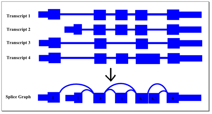
The thin exon sections represent untranslated regions (UTR) and the thick exon sections represent coding regions. Exons are drawn to scale and the connecting arcs represent splice paths. Each piece of transcript sequence is represented uniquely by a node, allowing each read to be aligned unambiguously within the splice graph so long as there are no redundant sequences within the exons themselves. When an exon has both long and short forms, it is split into two sub-exons such that the common portion is represented only once in the graph.
In this case, four transcript isoforms of a gene are collapsed into a single non-redundant splice graph. The gene would have 2 alternate promoter exons, exons 1 and 2, that both splice into exon 3. Exon 4 would be an alternative exon that is sometimes included and sometimes spliced out. Since Exon 5 has an two alternate 5’ donor sites, so it is split into sub-exons 5.1 and 5.2.
The SpliceSeqDBBuild process builds this reference set of splice graphs, one for each gene, using gene models downloaded from the UCSC Genome Browser database. Several different types of gene models are available, including RefSeq, UCSC Gene, Sanger Vega, Ensembl, and NCBI AceView, any of which may be used. Currently, SpliceSeq is distributed with splice graphs derived from Ensembl models because they tend to produce interpretable graphs with strong annotation and a nice balance between variation and complexity.
The steps performed by the SpliceSeqDBBuild are:
Use FTP to download gene model data from UCSC Genome Browser Tables. Currently, Ensembl (ensGene, ensPep, and ensemblToGeneName) is used.
Download chromosome sequence from NCBI.
Construct the SpliceSeq data schema.
For each gene, merge gene model transcripts into a single exon landscape map and splice list using genomic coordinates of each model exon.
Generate a consolidated splice graph for each gene. Split exons into sub-exons for contiguous regions with multiple points of splice in/out paths.
Annotate models with attributes for UTR, Coding, and transcript start/stop locations.
Retrieve and store nucleic sequence for each exon.
Download and store UniProt protein sequence and position specific feature information for each splice graph associate via gene symbol.
This reference set of splice graphs is then distributed together with the SpliceSeq package as SpliceSeq DB.
Alignment Sequence Database
Bowtie (first version) is used to align RNASeq reads to our database of splice graphs. The Bowtie alignment database is constructed from our splice graphs using a tiled window approach to create sequence records from each possible splice path within the window. Windows are used to control the combinatorial explosion that can occur when traversing the permutations of large genes with many alternative splice paths. The window size used to generate the Bowtie database is optimized based on sample read length (generally windows are 2x read length - 1 or 2x insert length – 1 for paired-end reads). Tiles are overlapped using a step size of the read length to ensure that a read falling at any position on the graph will be able to align.
A recursive graph traversal is performed to ensure that all paths are represented in the sequence database. Where possible, redundant sequence records are eliminated. The header of each sequence record is encoded with positional information about the exons and splice junctions contained in the sequence record. The header information allows quick identification of exons and junctions aligned to a given read in the Bowtie results. Even reads that cross multiple exons and splice junctions will align, allowing accurate measurement of exon and junction expression levels in regions with small exons and complex splicing patterns.
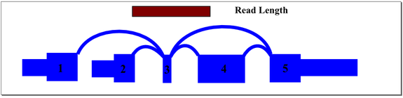
In the above example, mapping reads across exon 3 splice junctions is key to understanding the gene’s splice pattern, but exon 3 is too short to align to reads directly. A simple exon-exon splice junction database will also not align well because the exon 3 end of the junction will be too short to align fully with most reads that cross it. The approach we take in constructing the database includes all permutations of sequence that cross exon 3, optimized to match the sample read length. For this sample gene, database sequence would be generated for exon 1 to 3 to 4, exon 1 to 3 to 5, exon 2 to 3 to 4, and exon 2 to 3 to 5. Hence, a read of any location across exon 3 will align and be mapped to the appropriate junctions.
Detecting Novel Splices
Samples may contain transcripts not included in the original set of transcripts used to build the splice graph database. Sometimes, this means that the transcripts expressed by the sample may include splices that are not observed in the original splice graph. These splices are termed ‘novel’ splices. Some caution must be taken in this interpretation as the splice may be truly novel or it may be in a previously reported transcript record that was not in our source database (currently Ensembl)
In order to detect the presence of novel splices, we exhaustively generate all potential splice junctions between pairs of exons in a given gene that are not represented in the reference splice graph.
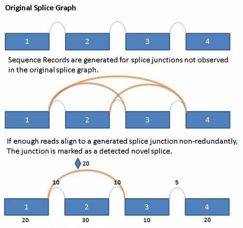
When reads are aligned to the primary alignment sequence database described above, the reads that do not align are saved to a separate file. These reads are then run in a second alignment step against a generated ‘novel’ junction sequence database. Reads that align with a minimum of 5 base overlap on both sides of the splice junction would be counted as an observation for the novel splice junction. When 3 or more reads with unique starting points align to a novel junction,then the ‘novel’ splice is considered to be observed and is added to the database. Novel splices are drawn in the splice graph like regular splices, but with a diamond symbol in the middle immediately above the arc.
The following diagram illustrates the process conceptually:
The limitation of the current method is that it does not detect exons that are not part of the original splice graph, and also does not address the possibility of novel alternate splice donor/acceptor junctions. This is a shortcoming that would be addressed by a later release of the software.
Single Sample Analysis
The first step in SpliceSeq analysis is to load one or more RNASeq samples. Sample reads are aligned to the splice graphs using Bowtie as described above.
Totals are collected for the number of times each exon or splice is observed. A read must include at least 4 bases of an exon to count as an observation for the exon and adjacent splice. (This minimum overlap value is configurable.) Note that a single read may traverse multiple exons and splices, allowing a read to contribute to the observation totals of multiple graph elements.
To obtain a normalized value that can be compared between samples, Exon/Splice totals are normalized by region length in 1000 bases (K) and by the total number of reads in the sample in millions (M). Normalized exon/splice totals are called “Observations Per Kilobases of exon/splice per Million aligned reads (OPKM)“.
Raw and normalized totals for exons, splices, and certain attributes are saved to the sample tables in SpliceSeq DB so that the load process needs only to be performed per sample.
Next, gene level analysis is done. Each gene’s expression level is computed in reads per kilobase of transcript length per million aligned reads (RPKM). Gene RPKM values count each read that uniquely maps to the gene once. The transcript length used for the RPKM calculation includes only exons that are expressed above a (configurable) background level of 25% of average exon expression. Gene expression levels are important for comparison processing when analyzing splicing difference between two samples.
After gene level RPKM values are calculated, a second pass is performed to allocate non-unique read alignments. Some reads can’t be uniquely aligned to a single gene. This happens most often in families of closely related genes because they contain regions of strong sequence similarity. If all non-unique reads are discarded, the splice graphs of genes that share sequence similarity will have “holes” in the graph where exons or splices are not able to get reads. This makes subsequent graph traversal for protein sequence analysis impossible.
To remedy this situation, we proportionally allocate degenerate reads based on the relative RPKM values of the genes to which the read aligns. For example, if there are 100 reads that align equally to exon 1 of gene A and exon 3 of gene B and gene A has an RPKM of 10 and gene B has an RPKM of 30, then 10/40 or ¼ of the 100 reads would be assigned as gene A exon 1 observations and 30/40 or ¾ of the 100 reads would be assigned as gene B exon 3 observations.
Next, a weighted recursive traversal of the graph is done to predict transcript and protein sequences that are likely to result from the observed exons and splices. If multiple transcript start exons have reads, they are weighted based on their relative OPKM values. For example, if one transcript start exon has an OPKM of 5, and an alternate start exon has an OPKM of 15, then the first gets a weight of 5/(5+15) = 25%. If alternate splice paths have reads, they are weighted in a similar fashion. By multiplying the weights of the start exon and alternate splices during traversal of the graph, we estimate a transcript level expression percentage. Transcript sequences are merged if they are identical, and they are discarded if the transcript expression level is less than 0.5%.
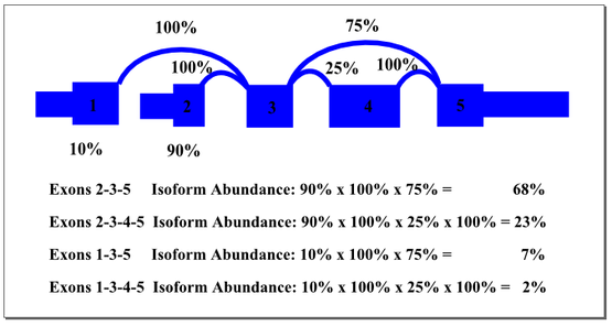
In the example above, there are two start exons and an alternative exon. The percentages shown in the graph represent the weighting of start exons and alternative splices based on observations from the reads. The most heavily weighted path starts with exon 2 and excludes the alternative exon 4. By multiplying the weights along that path, we find a predicted isoform prevalence of 68% for the sample. Other isoforms are weighted as indicated. It is possible that cellular mechanisms co-regulate splicing events that we treated by this method as independent. For example, maybe transcripts starting with exon 1 always include the alternate exon 4. In many cases, multiple splicing events are separated by more than the read length or insert length, making it impossible to identify co-regulation with current sequencing platforms. The SpliceSeq algorithm provides a good approximation of probable transcript composition and supports identification of significant shifts in splicing patterns that affect functional elements of the gene.
The transcript sequences produced by the weighted graph traversal are also translated into predicted protein sequence. The translation is done by identifying the start codon and translating the spliced sequence until a stop codon is encountered. Start codon identification is difficult because the first ATG is usually, but not always, the start codon. In constructing the splice graphs, we save the annotated start codon positions to take advantage of existing knowledge, rather than relying solely on computational methods. When conflicting start codons occur in the source gene models, the start codon with higher prevalence in the source gene models is used for translation. When stop codons occur 50+ base pairs upstream from a splice junction, the sequence is marked as a likely target for nonsense mediated decay. Redundant protein sequences are combined, and protein variant concentration estimates are summed from the original transcript concentration percentages.
The protein sequences produced in the preceding step are then aligned to the gene’s UniProt sequence. The alignment allows us to identify the portions of the UniProt sequence that are / are not included in a given protein variant and, by extension, which protein features are present / removed. UniProt annotations identify domains, motifs, structural elements, and binding regions that can help identify functional impacts of alternative splicing. By aligning the protein sequences modified by alternative splicing to the UniProt sequence, we can identify functional elements affected by splicing and can estimate the magnitude of the change from the variant’s concentration estimate. For example, in the case diagrammed below, a splice form estimated at 56% of the gene expression is lacking its localization signal peptide. UniProt features are characterized by type to allow filtering for splice events that affect certain types of protein features.
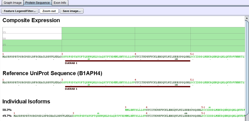
In this example, two proteins are produced by B1APH4. An alternate promoter removes some of the initial protein sequence in one variant. By aligning it to a canonical reference UniProt sequence, we see that the alternate promoter results in a partial loss of the protein’s KRAB-1 region.
Splice Event Detection
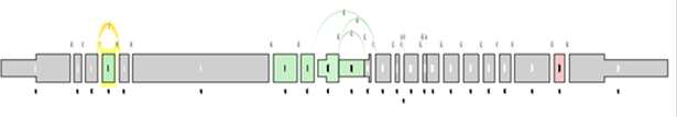
Next, the gene splice graph statistics are evaluated by a splice event detection module, which identifies and characterizes splice events. It identifies splice events such as alternate acceptor sites (AA), alternate donor sites (AD), alternate promoters (AP), alternate terminators (AT), exon skipping (ES), mutually exclusive exons (ME), and retained introns (RI) by analyzing the structure of the splice graph, looking for regions of the splice graph that can be traversed in multiple ways. The diagram below illustrates each event as represented within the splice graph.
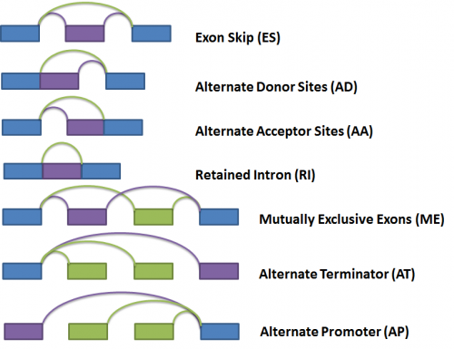
For the purposes of quantifying the event, we have arbitrarily labelled two types of paths for each event, one type being ‘inclusive’, meaning that a certain exon would be included if the path was traversed; and the other type being ‘exclusive’, meaning that a certain exon would be excluded if the path was traversed. In the diagram above, the inclusive path of each event type is colored in purple while the exclusive path(s) is colored in green.
For each event detected in a given sample, a value called called Percent-Spliced-In (PSI) is calculated for the event, which measures the proportion of reads falling on the ‘inclusive path’ as normalized by length. The actual formula is:
PSI = Inclusive reads / (inclusive reads + exclusive reads)
For instance, a PSI of 0.5 for an exon skip event would mean that the exon is included in half of the expressed isoforms, and a PSI of 0 would mean that the exon is never included in any of the transcripts.
Handling Complex Events
In the diagram above, only the simplest alternative splicing situations are listed. However, often times one can encounter complex regions in the splice graph which contains more than 2 alternative paths and can give rise to multiple splice events.
Consider the following splice graph structure:
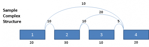
This complex graph structure gives 3 possible paths from Exon 1 to Exon 4. Depending on which pair of paths being examined, there are 3 possible splice events. Namely, exon skip of Exons 2 & 3 (ES 2,3), exon skip of Exon 2 (ES 2), and exon skip of Exon 3 (ES 3). Exons in these complex paths are often included in multiple possible paths. Calculations of PSI values and resulting p-values can be skewed if the read totals from an exon are included in all possible paths particularly when a path includes both heavy expression and weak expression exons. To address this issue for multi-exon events, the graph is broken out into separate paths, and the reads for each exon are proportionally allocated based on a weighted traversal of the graph segment involved. For the above example, this would mean:
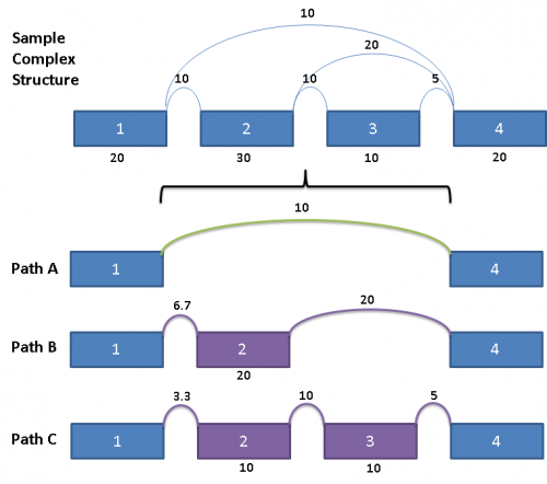
Each path from Exon 1 to Exon 4 have reads allocated to them proportionally, such that the sum of the paths A, B and C yields the read counts contained in the original splice graph.
The way they are allocated is as follows:
For Path A, since it does not share any exon or splice with Paths B and C, the reads count for the splice from Exon 1 to Exon 4 is the same as the original.
Paths B and C share the splice from Exon 1 to Exon 2, as well as Exon 2 itself. Since the outward going splices from Exon 2 (a splice from Exon 2 to Exon 3 and a splice from Exon 2 to Exon 4) are in the ratio of 1:2, the reads counts from the shared components are prorated to the same ratio as well.
Paths A, B, C gives rise to 3 splice events, namely exon skip of Exon 2 (Paths A & B), exon skip of Exons 2 & 3 (Paths A & C), as well as exon skip of Exon 3 (Paths B & C). The PSI for each of these events would then be calculated using the prorated read counts for each of these pairs of paths.
There is additional logic used to handle more complex graph structures, but the basic principle of separating the graph into different paths and allocating the aligned reads proportionally remains the same.
Compare Samples
A primary motivation for the construction of SpliceSeq was to assist in identification of alternative mRNA splicing that has biological relevance. A key goal, then, is the ability to compare samples and identify changes in splicing patterns that are likely to lead to protein alterations that affect function. Changes in the expression level of exons or splices is not indicative of alternate splicing if it simply reflects a change in overall gene expression level between the samples.
To identify and quantify changes in splicing patterns, we calculate the change in percent spliced in (PSI) values for each potential splice event in a gene. This value is also known as Delta PSI. The larger the absolute value of the delta PSI, the more significant the change in the splice event. For example, for a potential exon skip event with the following correct read values, the Delta PSI is calculated as follows:
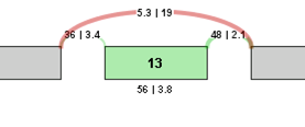
Delta PSI = PSI 2 - PSI 1 = (3.8/(19+3.8)) - (56/(56+5.3)) = 3.8/22.8 - 56/61.3 = 0.167 - 0.914 = -0.746
A p-value is also assigned to that event by using a 2-tailed Fisher’s exact test on a 2x2 contingency table of the raw inclusive and exclusive read counts for both samples.
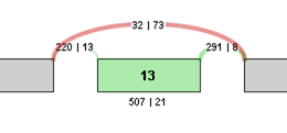
For example, the contingency table for the above Exon Skip example would be:
| Sample 1 | Sample 2 | |
|---|---|---|
| Inclusive reads | 507 | 21 |
| Exclusive reads | 32 | 73 |
The p-value for the event is less than 0.0001, making that event a highly significant difference between the 2 samples.
For visualization purposes, the log2 ratio of normalized read counts to gene expression level is calculated for each element of the graph. The log ratio provides a method of quantifying changes in expression of each exon/splice that is corrected for gene expression differences. The Log ratio indicates the magnitude of change and is a useful tool in coloring the graph red or green to identify splicing differences between samples.
Log ratio = log2 ((sample 1 exon OPKM / sample 1 gene RPKM) / (sample 2 exon OPKM / sample 2 gene RPKM))
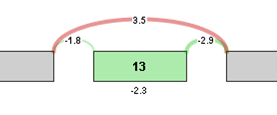
The coloring allows comparison of the splicing differences of individual components between the 2 samples. In the example above, we see that the long splice is more strongly expressed in sample 2 compared to sample 1, whereas exon 13 is expressed more strongly in sample 1 compared to sample 2. Therefore, sample 1 tends to express Exon 13 in its transcripts compared to sample 2.
The next step in the comparison analysis is to look for biological impacts of alternative splicing. Each gene is evaluated by comparing protein features of the two samples. When samples are imported into SpliceSeq, a prediction of protein sequence(s) is made based on the reads aligned to the splice graph. Each protein sequence is then aligned to UniProt to determine the protein features present. That comparison identifies changes in the % of protein features. For example, if a DNA binding site were present in 100% of the protein sequences produced by a gene in sample 1 but only 50% of protein sequences produced by the same gene in sample 2, it would be identified as a feature that changed because of splicing differences. Any feature with a difference in inclusion percentage above threshold is stored in the comparison database and presented in SpliceSeq as a ‘Uniprot Event’.
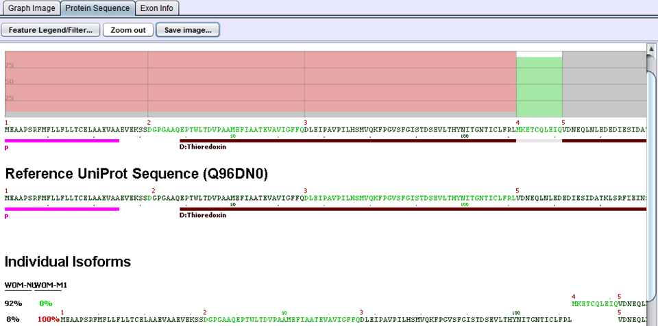
In the above example for the ERP27 gene, WOM-NU32 (sample 1) mostly expresses the first isoform starting at exon 4, whereas WOM-M1 (sample 2) only expresses the second isoform starting at exon 1. The inclusion of the Thioredoxin domain is 8% percent in sample 1 and 100% in sample 2. This gives rise to a delta PSI of 1.00 - 0.08 = 0.92
Groups
The ability to detect robust differences in splicing patterns increases when groups of samples are compared. SpliceSeq supports this type of analysis by allowing users to construct groups of samples. This is done during data loading by creating groups and specifying the member samples for each group. Prior to comparing groups, summary statistics for the group must be generated.
SpliceSeq group statistic generation involves traversing all the samples to establish summary statistics for every exon and splice for the group. These statistics are fairly simple. For each exon, and splice the average number of samples with reads, average number of reads, and average OPKM is calculated. If there are samples without reads for a given exon or splice, zero values for those samples are included in these averages so as not to skew averages of exons or splices with sparse coverage.
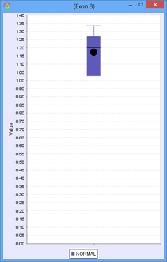
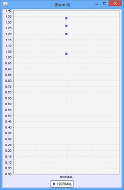
Consider the following part of a splice graph.
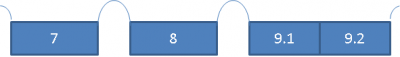
For a group containing 4 samples, each sample expresses Exon 8 at a different level. The scatter plot on the right would represent the raw normalized OPKM values for the exon, whereas the box plot on the left would represent the average values generated as the summary statistics for that exon. This process is done for every splice graph in the database.
Besides the above mentioned statistics, another important value that is also calculated is the ratio of OPKM to gene expression value (RPKM). Gene expression levels can vary across the samples so the best statistic to use in looking for splice variation is an expression adjusted value or the ratio of OPKM to gene level RPKM. This ratio is calculated for all exons and splices and the standard deviation of this value is also stored to assist with future statistical tests.
Gene level RPKM values are calculated for the group by averaging the RPKM values of each sample. The predicted percentage of each protein isoform is summarized by averaging concentrations from the samples in the group.
For each splice event, the PSI average and variance, as well as the number of participating samples are calculated. In cases where a sample does not express that gene, or if there is absolutely no activity in both the included and excluded paths of the splice event, that sample’s PSI is technically undefined. Therefore, that sample would not contribute to the PSI average and variance, and would be excluded from the number of participating samples instead.
Group level statistics for each gene are stored in the database. The group summary statistics can be examined using the Group View. Finally, the processes for identifying alternative splice events and protein impact described in the Single-Sample Analysis section above is performed for the group summary graphs.
Comparing Groups After groups have been summarized, they may be compared to identify statistically significant difference between the groups. The Compare Groups processing follows analytical steps similar to those described in the Compare Samples described above.
Every potential splice event is evaluated for group level splicing differences using the group level Delta PSI. Delta PSI for a group comparison is the difference in average PSI from each group. The p-value for delta PSI difference is calculated using a two-tailed t-test of unequal variance on the PSI values of the individual samples in the 2 groups.
There are also columns called “Group1 % Obs” and “Group 2 % Obs” that indicate the percentage of samples participating in the splice event from each group. In some cases coverage of a gene in some samples is so low that they are not used in the group statistics. When the splice event statistics are based on just a few members of a group, it may not be truly representative of a robust group level splicing event.
To illustrate this, we use the following example of an Exon skip event compared between 2 groups, ‘Normal’ and ‘Tumor’:
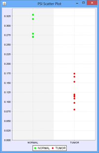
Every member sample of each group expressing that event would have a PSI, forming 2 distinct distributions of PSI values, 1 for each group. The Delta PSI is the difference between the average PSI of the Tumor group as compared to the normal group. The p-value is calculated using the PSI distribution of each group as the input. Given the separation of the 2 distributions, the p-value for this event is less than 0.0001 in this case. Since all the members of each group express the event, the “Group 1 %Obs” and “Group 2 %Obs” are both 100%.
The other group statistics generated to assist with filtering and interpretation of results are primary path and magnitude. In some complex splicing events, there are multiple possible paths under a splice with significant splicing differences. We calculate PSI values for all the possible paths but it simplifies interpretation to filter the event down to the dominant path (path with the most reads) under the differential splice. The path with the highest include read count is considered the primary path.
The magnitude value indicates the relationship between the splice event and overall gene expression. Sometimes there is a relatively large change in the splicing pattern on a portion of the graph that is very lightly expressed. Even though they are statistically significant, a very small percentage of transcripts of the gene are affected so it may make sense to filter these types of events out. The magnitude is simply a prediction of the percentage of isoforms that contain either of the alternative splice forms. A exon skip event with a magnitude of .01 indicates that the region of the splice graph containing the skip event was included in only 1% of transcripts.
At the level of the splice graph itself, for visualization purposes, the log2 ratio of average splice exon OPKM to gene expression RPKM is calculated. The log2 ratio is used in coloring of the individual elements of the graph red / green to indicate expression differences correct for differences in overall gene expression levels.
As in the case of sample comparison, green means enriched in the first group while red means enriched in the second group, and gray meaning there is no significant difference between the component expression level and overall gene expression level.