DeMixT
| Overview | |
| Description | Cell type-specific deconvolution of heterogeneous tumor samples with two or three components using expression data from RNAseq or microarray platforms |
| Development Information | |
| GitHub | wwylab/DeMixT |
| Language | R (package), HTML (website) |
| Current version | 1.14.0 |
| License | Artistic (package) |
| Status | Active |
| Last updated | 2022/10/13 |
| References | |
| Citation | Wang, Z., Cao, S., Morris, J.S., Ahn, J., Liu, R., Tyekucheva, S., Gao, F., Li, B., Lu, W., Tang, X. and Wistuba, I.I., Bowden, M., Mucci, L., Loda, M., Parmigiani, G., Holmes, C., Wang, W. (2018). Transcriptome Deconvolution of Heterogeneous Tumor Samples with Immune Infiltration. iScience, 9, pp.451-460. https://doi.org/10.1016/j.isci.2018.10.028 |
| Help and Support | |
| Contact |
Shaolong Cao
Peng Yang Wenyi Wang |
| Discussion | Issues on GitHub |
DeMixT
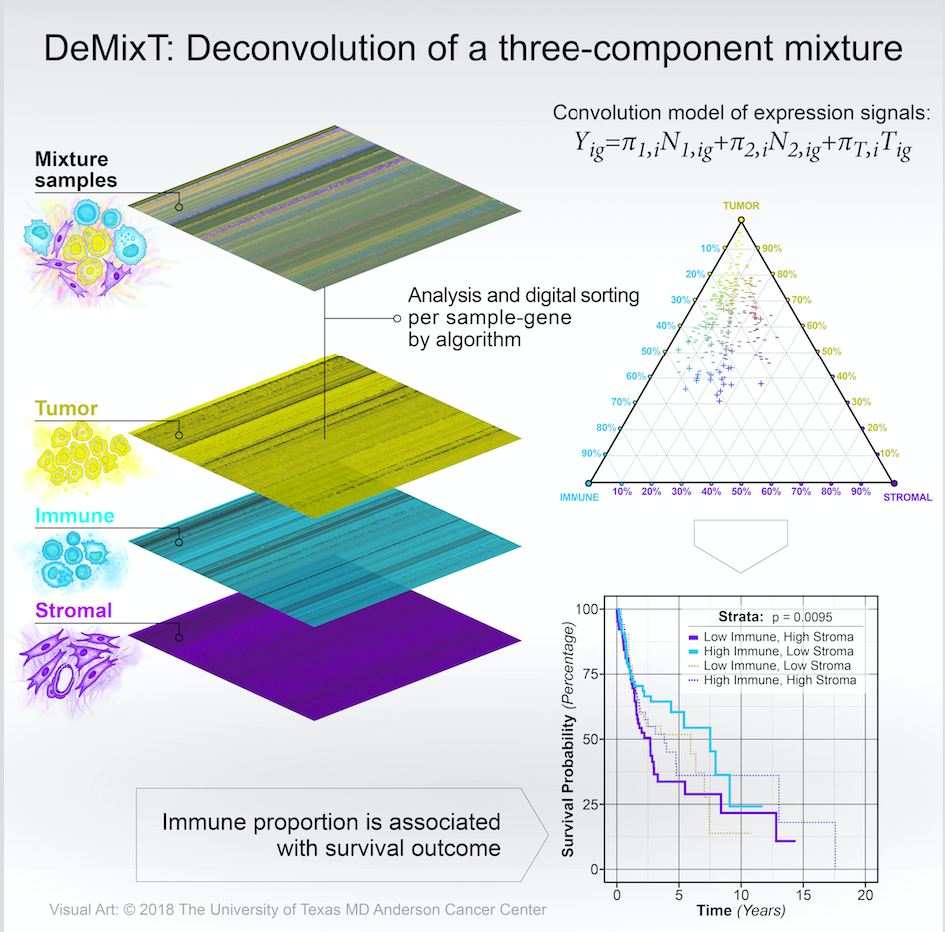
Transcriptomic deconvolution in cancer and other heterogeneous tissues remains challenging. Available methods lack the ability to estimate both component-specific proportions and expression profiles for individual samples. We develop a deconvolution model, DeMixT, for expression data from a mixture of cancerous tissues, infiltrating immune cells and tumor microenvironment. DeMixT is a software package that performs deconvolution on transcriptome data from a mixture of two or three components.
DeMixT 1.14.0 is updated with the following changes:
Added preprocessing functions and modified vignettes accordingly.
Included R.h in DeMixT.c to fix compilation error caused by Rprintf.
Fixed the logic operation in the IF_inverse function of DeMixT_GS.
Installation
The DeMixT package is compatible with Windows, Linux and MacOS. The user can install it from Bioconductor:
if (!require("BiocManager", quietly = TRUE))
    install.packages("BiocManager")

BiocManager::install("DeMixT")
For Linux and MacOS, the user can also install the latest DeMixT from GitHub:
if (!require("devtools", quietly = TRUE))
    install.packages('devtools')

devtools::install_github("wwylab/DeMixT")
Check if DeMixT is installed successfully:
# load package
library(DeMixT)
Note: DeMixT relies on OpenMP for parallel computing. Starting from R 4.00, R no longer supports OpenMP on MacOS, meaning the user can only run DeMixT with one core on MacOS. We therefore recommend the users to mainly use Linux system for running DeMixT to take advantage of the multi-core parallel computation.
For the details about the functions in DeMixT package, please refer to the Manual .
Example (version 1.14.0)
Simulated two-component data
Estimate proportions for simulated two-component data with spike-in normal reference.
data("test.data.2comp")
res.GS = DeMixT_GS(data.Y = test.data.2comp$data.Y,
data.N1 = test.data.2comp$data.N1,
niter = 30, nbin = 50, nspikein = 50,
if.filter = TRUE, ngene.Profile.selected = 150,
mean.diff.in.CM = 0.25, ngene.selected.for.pi = 150,
tol = 10^(-5))
## Read the results
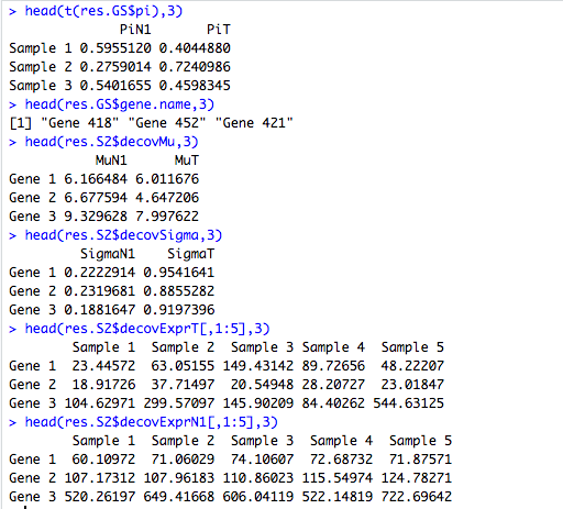
head(t(res.GS$pi),3)
head(res.GS$gene.name,3)
## Two-component deconvolution given proportions
res.S2 <- DeMixT_S2(data.Y = test.data.2comp$data.Y,
data.N1 = test.data.2comp$data.N1,
data.N2 = NULL,
givenpi = c(t(res.S1$pi[-nrow(res.GS$pi),])), nbin = 50)
head(res.S2$decovMu,3)
head(res.S2$decovSigma,3)
head(res.S2$decovExprT[,1:5],3)
head(res.S2$decovExprN1[,1:5],3)DeMixT returns a list object. The res.GS\$pi is a matrix of estimated proportions for each component (in columns) and each sample (in rows). The res.S2\$deconvExprT, res.S2\$deconvExprN1 (and res\$deconvExprN2 if the 3-component model is chosen) are matrices of deconvolved expression profiles corresponding to the unknown T-component and known N1-component (and N2-component), respectively. The res.S2\$deconvMu and res.S2\$deconvSigma are two matrices of estimated $\mu$ and $\sigma$ for each component (in columns) and each gene (in rows).
Real data: PRAD in TCGA dataset
1. Preprocessing
For the deconvolution of real data with DeMixT, the user may apply the following preprocessing steps first. Here, we use the PRAD (prostate adenocarcinoma) from TCGA as an example.
- (Optional) Remove suspicious samples by hierarchical clustering
It is possible that the some of the tumor and normal samples are mislabelled. We use the function
# hc_labels <- detect_suspicious_sample_by_hierarchical_clustering_2comp(count.matrix, normal.id, tumor.id)
to visually inspect the separation of tumor and normal samples based on the hierarchical clustering of their expressions, in which count.matrix is the raw count matrix; normal.id and tumor.id are the vectors of normal and tumor sample ids, respectively. Generally, one cluster contains tumor samples and the other contains normal samples. Any samples that are clustered outside of its own group label, e.g., tumor samples clustered within the normal sample cluster or normal samples in the tumor cluster, are considered as mislabelled samples and filtered out.
knitr::include_graphics(path = paste0("hierarchical_clustering.png"))count.matrix, normal.id and tumor.id are updated by
# normal.id <- setdiff(normal.id, names(hc_labels$cluster[hc_labels$cluster == 1]))
# tumor.id <- setdiff(tumor.id, names(hc_labels$cluster[hc_labels$cluster == 2]))
# count.matrix <- count.matrix[, c(normal.id, tumor.id)]- Select genes with small variation in gene expression across samples
In this step, we select a subset of ~9000 genes from the original gene set (>50,000) before running DeMixT with the GS (Gene Selection) method so that our model-based gene selection maintains good statistical properties. We use the function
# plot_sd(count.matrix, normal.id, tumor.id)
to visualize the distribution of standard deviation of log2 expressions space of normal and tumor samples,
knitr::include_graphics(path = paste0("sd_expresion.png"))and use the function
# num_gene_remaining_different_cutoffs <- subset_sd_gene_remaining(count.matrix, normal.id, tumor.id, cutoff_normal_range = c(0.1, 1.0), cutoff_tumor_range = c(0, 2.5), cutoff_step = 0.1)
to find he a range of variance in genes from normal samples (cutoff_normal_range) and from tumor samples (cutoff_tumor_range) which results in roughly 9,000 genes.
We then use the function
# count.matrix <- subset_sd(count.matrix, normal.id, tumor.id, cutoff_normal = cutoff_normal_range, cutoff_tumor = cutoff_tumor_range)
to update the count.matrix such that it only includes the selected genes.
- Scale normalization
We apply a scale normalization at the 75th percentile across all the tumor and normal samples using the function
# count.matrix <- scale_normalization_75th_percentile(count.matrix)
to adjust the expression levels in the samples.
Note: The user may also use the function
# count.matrix <- DeMixT_preprocessing(count.matrix, normal.id, tumor.id, cutoff_normal_range = c(0.1, 1.0), cutoff_tumor_range = c(0, 2.5), cutoff_step = 0.1)
to perform the preprocessing steps of 2) and 3) in one go.
- (Optional) Batch effect correction for tumor samples from different batches by ComBat
If the tumor samples are from different batches, we recommend the user to inspect the batch effect using the function before running DeMixT
# plot_dim(count.matrix.tumor, labels, legend.position = 'bottomleft', legend.cex = 1.2)
This function will generate a PCA plot, in which the samples are colored by the labels indicating different batches of tumor samples, as well as normal samples. If there is a clear separation between different batches of tumor samples, there is likely batch effects. We use the function
# count.matrix.tumor <- batch_correction(count.matrix.tumor, labels)
to reduce this effect, where count.matrix.tumor is the raw count matrix only from tumor samples and labels is the factor of tumor batches. The user may choose other batch effect correction methods at this step.
The user may inspect the batch effect again after the above step using the mentioned function
# plot_dim(count.matrix.tumor, labels, legend.position = 'bottomleft', legend.cex = 1.2)
2. Deconvolution using DeMixT
To optimize the DeMixT parameter setting for the input data, we recommend testing an array of combinations of the number of spike-ins and the number of selected genes.
The number of CPU cores used by the DeMixT function for parallel computing is specified by the parameter nthread. By default (such as in the code block below), nthread = total_number_of_cores_on_the_machine - 1. The user can change nthread to a number between 0 and the total number of cores on the machine.
## Because of the random initial values and the spike-in samples within the DeMixT function,
## we would like to remind the user to set seeds to keep track. This seed setting will be
## internalized in DeMixT in the next update.

# set.seed(1234)

# data.Y = SummarizedExperiment(assays = list(counts = count.matrix[, tumor.id]))
# data.N1 <- SummarizedExperiment(assays = list(counts = count.matrix[, normal.id]))

## In practice, we set the maximum number of spike-in as min(n/3, 200),
## where n is the number of samples.
# nspikesin_list = c(0, 50, 100, 150)
## One may set a wider range than provided below for studies other than TCGA.
# ngene.selected_list = c(500, 1000, 1500, 2500)

#for(nspikesin in nspikesin_list){
#    for(ngene.selected in ngene.selected_list){
#        name = paste("PRAD_demixt_GS_res_nspikesin", nspikesin, "ngene.selected",
#                      ngene.selected,  sep = "_");
#        name = paste(name, ".RData", sep = "");
#        res = DeMixT(data.Y = data.Y,
#                     data.N1 = data.N1,
#                     ngene.selected.for.pi = ngene.selected,
#                     ngene.Profile.selected = ngene.selected,
#                     filter.sd = 0.7, # same upper bound of gene expression standard deviation
#                     # for normal reference. i.e., preprocessed_data$sd_cutoff_normal[2]
#                     gene.selection.method = "GS",
#                     nspikein = nspikesin)
#        save(res, file = name)
#    }
#}
We suggest selecting the optimal parameter combination that produces the largest average correlation of estimated tumor propotions with those produced by other combinations. The location of the mode of the Pi estimation may also be considered. The mode located too high or too low may suggest biased estimation.
Instead of selecting using the parameter combination with the highest correlation, one can also select the parameter combination that produces estimated tumor proportions that are most biologically meaningful.
A comprehensive tutorial of using DeMixT for real data deconvolution can be found at https://wwylab.github.io/DeMixT/tutorial.html.
Knitr documentation for all analyses performed in the DeMixT manuscript[1] can be found here .
Reference
[1]. Wang, Z. et al. Transcriptome Deconvolution of Heterogeneous Tumor Samples with Immune Infiltration. iScience 9, 451–460 (2018).
Support
For questions or support related to the use of either the DeMixT R package or web app, please visit the project on GitHub .
For other inquiries, please contact
Wenyi Wang
.
Legalese
This website is for educational and research purposes only.